Hiranmay's WebDiary

An apparent inconsistency in the atomic transition

In 1913, while correcting the flaws of Rutherford's model of atoms, Bohr assumed few counterintuitive facts in ad-hoc manner. Few of those assumptions were the following,

Though the assumptions seems to come from nowhere, they were actually motivated by the observation of pecularity of emission and absorption spectra of hydrogen atoms (see figure 1). Both of these spectrum have only few lines and that forced Bohr to take those aforementioned assumptions.

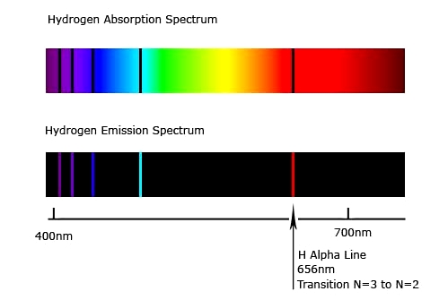
Fig.1 The famous Hydrogen Spectra.

While the emission spectra is quite persuadable, the absorption spectra raise one simple doubt, why is the light having higher frequency \(\nu'\) than required (\(\nu\)), not absorbed by the electron? A simple mind would rather intuit that it's more likely for a higher energy photon to cause the excitation by supplying a part of its energy to the electron, but it doesn't happen in nature as suggested by the absorption spectra. The question is why?

Well, the explanation involves little advanced quantum mechanics (the word 'advanced' has been used in relative sense) to be more specific, time dependent perturbation theory (TDPT). Here it is,

I think it's better to start from our familiar Schrodinger equation, \begin{equation} i\hbar \frac{\partial \Psi(r,t)}{\partial t} = \left [ -\frac{\hbar^2}{2m} \nabla^2 + V(r,t) \right]\Psi(r,t) \label{eq:se} \end{equation} where, \( \psi \) is called the wave-function of the system, \( V(r,t) \) is the potential. Often the term inside the squared bracket is written as \(H\) and interpreted as the Hamiltonian of the system. Now, if we assume that \( \Psi \) can be written as product of a spatial function and a time dependent function only, i.e. $$ \Psi(r,t) = \psi(r) \phi(t) $$ It can be shown by substituting the value of \(\Psi\) in equation \eqref{eq:se}, the following relations hold, \begin{equation} \phi(t) = e^{-iEt/\hbar} \end{equation} and, \begin{equation} \left [ -\frac{\hbar^2}{2m} \nabla^2 + V(r,t) \right]\psi(r) = E\psi(r) \label{eq:tise} \end{equation} or, $$ H\psi(r) = E \psi(r) $$ Equation \eqref{eq:tise} is called the time independent Schrodinger equation where \( E \) is interpreted as the energy of the particle/system. Wave-functions (or states), \(\psi\) that satisfy this equation is called the eigen-states of the Hamiltonian.These eigen states in Bohr's language are different atomic orbitals. Eigen states are also called stationary states, because if an electron is in any of these eigen states, they stay there forever as long as the Hamiltonian is unchanged. Now, combining the functions, \(\psi(r)\) and \( \phi(t) \), we get the actual wavefunction as, $$ \Psi = \psi(r)e^{-iEt/\hbar} $$

One peculiar fact about the quantum world is that, the electrons can be in more than one states until you observe them. In quantum physics we rather say the electronic state is a superposed state of more than one states. The very moment you observe the electrons, they will go to any of those aforementioned eigen states and will pretend that they were at this state from the begining. But if you take a number of identical systems and observe all of them, you will see that the electrons are at different states in different system although they were identical. A way to mathematically represent these kind of mixed states is expressing them as linear combination of different states, i.e. $$ \Psi(r,t) = c_1\Psi_1(r,t) + c_2\Psi_2(r,t) + c_3 \Psi_3(r,t) + .. $$ Different states may be of different energies, so the time part of those wavefunctions will vary. So, the states will evolve with time according to the following relation, $$ \Psi(r,t) = c_1\psi_1(r) e^{-iE_1t/\hbar} + c_2\psi_2e^{-iE_2t/\hbar} + .. $$ Now, let us take only two such states for simplicity, say \(\psi_a\) and \(\psi_b\) and also assume that their energies are \(E_a\) and \(E_b\). Furthermore consider that the electron is in a superposition of these two different states, mathematically, $$ \psi(0) = c_a\psi_a + c_b\psi_b $$ At this point we need to emphesize the significance of this coefficients \(c_a\) and \(c_b\). If these coefficients are normalized, or in other words, \( |c_a|^2 + |c_b|^2 = 1 \), the probability that the electron will be in state \(\psi_a\), if observed, is, $$ P_a = |c_a|^2 $$ Similarly the electron will be in state \(\psi_b\) with probability, $$ P_b = |c_b|^2 $$ As, \(\psi_a\) and \(\psi_b\) are eigen states, according to the time independent Schrodinger equation, $$ \hat{H_0}\psi_a = E_a\psi_a,\; \; \hat{H_0}\psi_b = E_b\psi_b $$ And the state \(\psi\) will evolves with time, according to the following relation, $$ \psi(t) = c_a\psi_a e^{-iE_at/\hbar} + c_b\psi_be^{-iE_bt/\hbar} $$ \( c_a \) and \(c_b\) are constant as long as the Hamiltonian is unchanged. Now, if we introduce a time dependent perturbation in the potential \(V\), the resultant Hamiltonian would be, $$ \hat{H} = \hat{H_0} + \hat{H'}(t) $$ The time dependent nature of the Hamiltonian makes the coefficients, \(c_a\) and \( c_b\) change with time and the relation is the following ( sorry to state it directly, the derivation would just make the discussion cumbersome, if you wish you can skip this part), $$ \frac{dc_a}{dt} = -\frac{i}{\hbar}H'_{ab}e^{-i\omega_0t}c_b $$ $$ \frac{dc_b}{dt} = -\frac{i}{\hbar}H'_{ba}e^{-i\omega_0t}c_a $$ Where, $$ H'_{ab}\equiv \bra{\psi_a}H'\ket{\psi_b} $$ $$ H'_{ba}\equiv \bra{\psi_b}H'\ket{\psi_a} $$ and, $$ \omega_0 = \frac{E_b - E_a}{\hbar} $$ One thing to notice is that the above equation is a coupled differential equation. A good starting point to unravel the usefulness of the above equation would be considering \(c_a = 1\) and \(c_b = 0\), i.e. assuming the electron starts from the state \(\psi_a\). Substituting the value of \(c_a\) and \(c_b\) in the above equation we get the first order correction, $$ \frac{dc_a^{(1)}}{dt} = 0 $$ \begin{equation} c_a^{(1)}(t) = 1 \end{equation} $$ \frac{dc_b^{(1)}}{dt} = -\frac{i}{\hbar}H'_{ba}e^{i\omega_0t} $$ \begin{equation} c_b^{(1)}= -\frac{i}{\hbar}\int_0^t H'_{ba}(t')e^{i\omega_0t'}dt' \label{eq:change} \end{equation} substituting the first order values of this equation again in the previous equation, we get the second order correction and continuing in this manner we get all the higher order corrections.

Even if you don't understand the above mathematical formulation, it hardly matters. What important is, because of the time dependent potential, \(c_a\) and \(c_b\) are no longer constant, rather they change with time. And their change is described by the equation \eqref{eq:change}. That's all about the formalism, now let's focus on our specific problem, a perturbation caused by incident light (or EM wave). For the sake of simplicity, we will assume that the incident wave is sinusoidal which introduces a cosine potential (perturbation) inside the atom ( as, \(E = -\nabla V\) ), i.e. $$ H'(\mathbf{r},t) = V(\mathbf{r})\cos{(\omega t)} $$ so that, $$ H'_{ab} = V_{ab}\cos{(\omega t)} $$ where, $$ V_{ab} \equiv \bra{\psi_a}V(\mathbf{r})\ket{\psi_b} $$ Note that, \(\omega\) is nothing but the angular frequency of the incident photon/light wave. Performing the integration as shown in equation \eqref{eq:change}, with limit 0 to t, we get, $$ c_b(t) \approx - \frac{V_{ba}}{2\hbar}\left[\frac{e^{i(\omega_0 + \omega)t} - 1}{\omega_0 + \omega} + \frac{e^{i(\omega_0 - \omega)t} - 1}{\omega_0 - \omega} \right] $$ This may seem complicated but, physicists have an excellent tool to simplify stuffs, it's called approximation. Since we already know the fact that the emission/ absorption takes place when \(\omega\) is roughly same as \(\omega_0\), it is sufficient to investigate the effect of the perturbation for \(\omega \approx \omega_0 \). So that, $$ |\omega_0 + \omega| >>|\omega_0 - \omega| $$ which encourages us to neglect the first term inside the square bracket. Now, the expression becomes, \begin{equation} c_b(t) \approx - \frac{V_{ba}}{2\hbar}\left[ \frac{e^{i(\omega_0 - \omega)t} - 1}{\omega_0 - \omega} \right] = -i\frac{V_{ba}}{\hbar}\frac{\sin{\left[(\omega_0 - \omega)t/2\right]}}{\omega_0 - \omega} \end{equation} A remarkable result indeed. So, the probability of finding the electron in the state \(\psi_b\) is simply, \begin{equation} P = |c_b|^2 \approx \frac{|V_{ab}|^2}{\hbar^2}\frac{\sin^2{\left[(\omega_0 - \omega)\right]t/2}}{(\omega_0 - \omega)^2} \label{eq:final} \end{equation} Now, if you remember, we started with the state \(\psi_a\) only, and we are getting a positive probability for the electron to be in state \(\psi_b\). In other words, there is a chance of transition from the state \(\psi_a\) to \(\psi_b\). That's why \(P\) is called transition probability. But did we get our answer? No, we will if we plot the transition probability vs \( \omega \) graph. In the figure (2), you can easily see that the transition probability is much larger at the vicinity of \(\omega = \omega_0\). That explains why the transition is caused by mostly the light of a certain frequency (\(\nu\)). Although the transition probability is very less for higher or lower frequency than \(\omega_0\), it's not zero except few points, so you can still get transition for those wavelengths, but the chance is very less. An interesting point to be noted is that, the graph is symmetric, so if you are little brave you would say, that an EM wave having less frequency than \(\nu\) is also capable of causing the excitation. Really!!

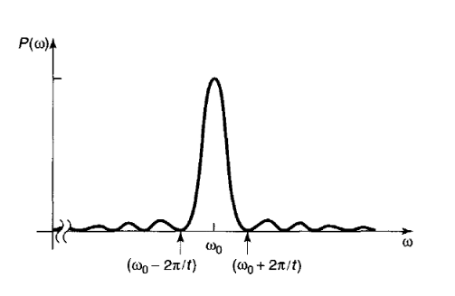
Fig.2 Angular frequency vs. Transition probability graph.

Another doubt may come to your mind regarding the transition probability, In our assumption there was nothing special about the states, we didn't mention which states is the lower energy state, and which one is higher. So, this analysis is equally applicable for the transition from higher energy state to lower energy state, and suggests an emission due to presence of radiation. These phenomena are called stimulated emission and it reveals why the electron goes from higher energy states to lower energy states. But it again raise an annoying question, what if the electron is already in higher energy state and the whole system is kept in dark, i.e. in the absence of radiation, will the transition still happen? The answer is yes, and it was known as spontaneous emission. But isn't it against the law of quantum mechanics because, without the perturbation, the electrons are supposed to stay wherever they are? No, because there is no such thing as purely spontaneous emission. Without perturbation, the electron would stay in the higher energy state for eternity. However in quantum electrodynamics the fields are nonzero even in the ground states, just like the ground state energy of the harmonic oscillator is nonzero. So, whatever you do, wherever you go, there will always be radiation to cause the perturbation and will encourage the electron to break its commitment to the excited state.

I had this doubt since my school days, and finally got the explanation while reading time dependent perturbation theory from Griffith's Quantum Mechanics book. I have skipped the derivations to keep this discussion short, if you want you can read the Chapter 9 of this book. In case you find any mistake in the above discussion, please let me know.

References

[1] Griffiths, D.J. and Schroeter, D.F., 2018. Introduction to quantum mechanics. Cambridge University Press.

[2] Sakurai, J.J. and Napolitano, J., 2014. Modern quantum mechanics (Vol. 185). Harlow: Pearson.